HomographyNet: Deep Image Homography Estimation

Introduction

Today we are going to talk about a paper I read a month ago titled Deep Image Homography Estimation. It is a paper that presents a deep convolutional neural network for estimating the relative homography between a pair of images.

What is a Homography?

In projective geometry, a homography is an isomorphism of projective spaces, induced by an isomorphism of the vector spaces from which the projective spaces derive. - Wikipedia

If you understood that, go ahead and skip directly to the deep learning model discussion. For the rest of us, let’s go ahead and learn some terminology. If you can forget about that definition from Wikipedia for a second, let’s use some anologies to at least get a high-level idea.

Isomorphism?

If you decide to bake a cake; the process of taking the ingredients and following the recipe to create the cake could be seen as morphing. The recipe allowed you to morph/transition from ingredients to a cake. If you’re thinking wtf, just stick with me a bit longer. Now, imagine the same recipe could allow you to take a cake and morph/transition back to the ingredients if you follow it in reverse! In a nutshell, that is the definition of an isomorphism. A recipe that can allow you to transition between the two, loosely speaking.

Isomorphism in mathematics is morphism or a mapping (recipe) that can also give you the inverse, again loosely speaking.

Projective geometry?

I don’t have a clever analogy here, but I’ll give you a simple example to tie it all together. Imagine you’re driving and your dash cam snapped a picture of the road in front of you (let’s call this pic A); at the same time, imagine there was a drone right above you and it also took a picture of the road in front of you (let’s call this pic B). You can see that pic A and B are related, but how? They’re both pictures of the road in front you, only difference is the perspective! The big question….

Is there a recipe/isomorphism that can take you from A to B and vice versa?

There you go, the question you just asked is what a Homography tries to answer. Homography is an isomorphism of perspectives. A 2D homography between A and B would give you the projection transformation between the two images! It is a 3x3 matrix that descibes the affine transformation. Entire books are written on these concepts, but hopefully we now have the general idea to continue.

NOTE

There are some constraints about a homography I have not mentioned such as:

1. Usually both images are taken from the same camera.
2. Both images should be viewing the same plane.

Motivation

Where is homography used?

To name a few, the homography is an essential part of the following

• Creating panoramas
• Monocular SLAM
• 3D image reconstruction
• Camera calibration
• Augmented Reality
• Autonomous Cars

How do you get the homography?

In traditional computer vision, the homography estimation process is done in two stages.

1. Corner estimation
2. Homography estimation

Due to the nature of this problem, these pipelines are only producing estimates. To make the estimates more robust, practitioners go as far as manually engineering corner-ish features, line-ish features etc as mentioned by the paper.

Robustness is introduced into the corner detection stage by returning a large and over-complete set of points, while robustness into the homography estimation step shows up as heavy use of RANSAC or robustification of the squared loss function. - Deep Image Homography Estimation

It is a very hard problem that is error-prone and requires heavy compute to get any sort of robustness. Here we are, finally ready to talk about the question this paper wants to answer.

Is there a single robust algorithm that, given a pair of images, simply returns the homography relating the pair?

HomographyNet: The Model

HomographyNet is a VGG style CNN which produces the homography relating two images. The model doesn’t require a two stage process and all the parameters are trained in an end-to-end fashion!

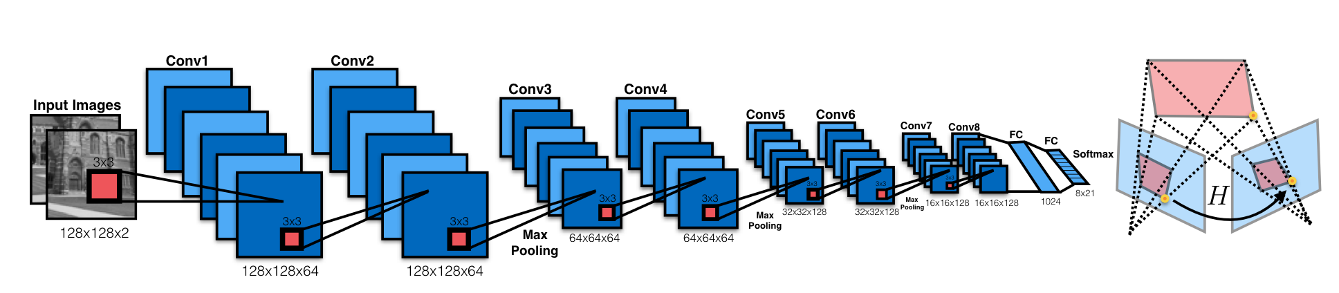
HomographyNet as descibed in the paper comes in two flavors, classification and regression. Based on the version you decide to use, they have their own pros and cons. Including different loss functions.

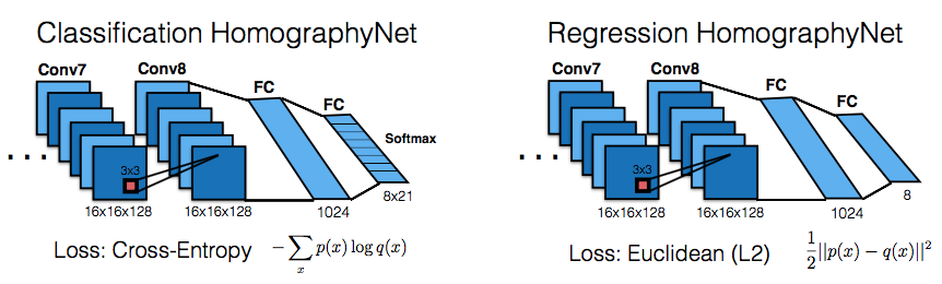
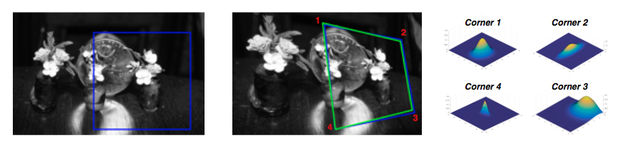
The regression network produces eight real-valued numbers and uses the Euclidean (L2) loss as the final layer. The classification network uses a quantization scheme and uses a softmax as the final layer. Since they stick a continuous range into finite bins, they end up with quantization error; hence, the classification network additionally also produces a confidence for each of the corners produced. The paper uses 21 quantization bins for each of the eight output dimensions, which results in a final layer of 168 output neurons. Each of the corner’s 2D grid of scores are interpreted as a distribution.

The architecture seems simple enough, but how is the model trained? Where is the labeled dataset coming from? Glad you asked!

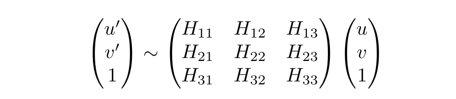
As the paper states and I agree, the simplist way to parameterize a homography is with a 3x3 matrix and a fixed scale. In the 3x3 homography matrix, [H11:H21, H12:H22] are responsible for the rotation and [H13:H23] handle the translational offset. This way you can map each pixel at position [u,v,1] from the image against the homograpy like the figure below, to get the new projected transformation [u',v',1].

However! If you try to unroll the 3x3 matrix and use it as the label (ground truth), you’d end up mixing the rotational and translational components. Creating a loss function that balances the mixed components would have been an unnecessary hurdle. Hence, it was better to use well known loss functions (L2 and Cross-Entropy) and instead figure out a way to re-parameterize the homography matrix!

The 4-Point Homography Parameterization

The 4-Point parameterization is based on corner locations, removing the need to store rotational and translation terms in the label! This is not a new method by any means, but the use of it as a label was clever! Here is how it works.

Earlier we saw how each pixel [u,v,1] was transformed by the 3x3 matrix to produce [u',v',1]. Well if you have at least four pixels where you calculate delta_u = u' - u and delta_v = v' - v then it is possible to reconstruct the 3x3 homography matrix that was used! You could for example use the getPerspectiveTransform() method in OpenCV. From here on out we will call these four pixels (points) as corners.

Training Data Generation

Now that we have a way to represent the homography such that we can use well known loss functions, we can start talking about how the training data is generated.

As a sidenote, H^AB denotes the homorgraphy matrix between A and B

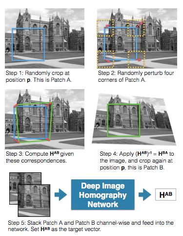
Creating the dataset was pretty straightforward, so I’ll only highlight some of the things that might get tricky. The steps as the describe in the above figure are:

1. Randomly crop a 128x128 patch at position p from the grayscale image I and call it patch A. Staying away from the edges!
2. Randomly perturb the four corners of patch A within the range [-rho, rho] and let’s call this new position p'. The paper used rho=32
3. Compute the homography of patch A using position p and p' and we’ll call this HAB
4. Take the inverse of the homography (HAB)^-1 which equals HBA and apply that to image I, calling this new image I'. Crop a 128x128 patch at position p from image I' and call it patch B.
5. Finally, take patch A and B and stack them channel-wise. This will give you a 128x128x2 image that you’ll use as input to the models! The label would be the 4-point parameterization of HAB.

They cleverly used this five step process on random images from the MS-COCO dataset to create 500,000 training examples. Pretty damn cool (excuse my english).

The Code

If you’d like to see the regression network coded up in Keras and the data generation process visualized, you’re in luck! Follow the links below to my Github repo.

• HomographyNet Regression variant
• Dataset Generation Visualization

Final thoughts

That pretty much highlights the major parts of the paper. I am hoping you now have an idea of what the paper was about and learned something new! Go read the paper because I didn’t talk about the results etc.

I’d like to think easy future improvements could be to swap out the heavy VGG network for squeezenet! Giving you the improvement of a smaller network. I’ll maybe experiment with this idea and see if I can match or improve on their results. As for possible uses today, I could see this network being used as a cascade classifier. The traditional methods are very compute heavy, so if we could maybe have this network in front to filter out the easy wins, we could cut down on compute cost.

Stay tuned for the next paper and please comment with any corrections or thoughts. That is all folks!